Rasters in R

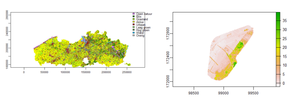
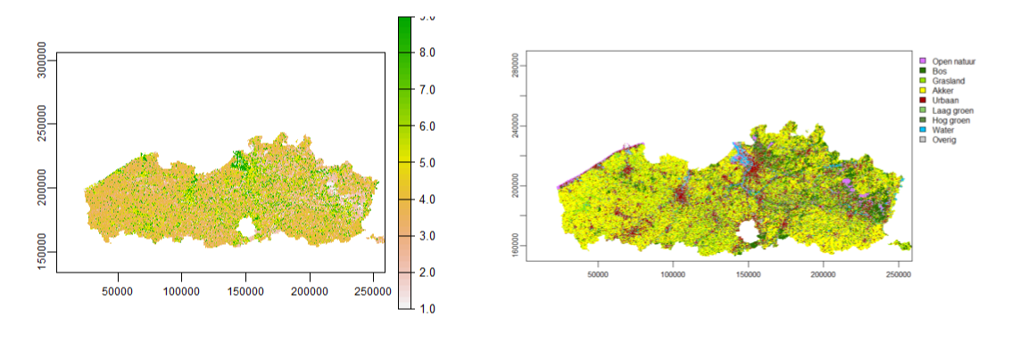
class: center, top

![:scale 30%](/assets/images/coding_club_logo_1.png)

<!-- Adjust the presentation to the session. Focus on the challenges,
this is not a coding tutorial.

Note, to include figures, store the image in the `/docs/assets/images`
folder and use the jekyll base.url reference as done in this template
or see https://jekyllrb.com/docs/liquid/tags/#links.
  using the scale attribute ![:scale 30%](...), you can adjust the image size.
-->

# 24 NOVEMBER 2022

## INBO coding club

Herman Teirlinck<br>
01.17 - Clara Peeters

---
class: left, top

## ROOMIE: room reservation

```
> if (isFALSE(roomie)) {
+   warning("Please confirm asap the room reservation on the roomie")
+ }
Warning message:
Please confirm asap the room reservation on the roomie
```

---
class: left, top

## Introduction: open software

![:scale 100%](/assets/images/20221124/20221124_quote_about_arcgis.png)

---
class: center, middle

![:scale 90%](/assets/images/20221124/20221124_rasters_badge.png)

---
class: left, top

## raster, terra, stars, sf, sp, ... HELP!

R is rapidly evolving to fill the gap with Python and C++. Downside: new packages are being developed, old ones are modified or superseded.

### Spatial vector data

Topic of the coding club of October

- **sf** : newest and recommended package
- **sp** : its predecessor

### Spatial raster data

- [**terra**](https://rspatial.github.io/terra/reference/terra-package.html) : newest and recommended package
- [**raster**](https://rspatial.org/raster/pkg/index.html) : its predecessor (no support for sf), match with sp
- [**stars**](https://r-spatial.github.io/stars/) : for **s**patio**t**emporal **ar**ray**s**

For more info, read this great [article](https://geocompr.github.io/post/2021/spatial-classes-conversion/) about conversions among different spatial classes in R.

---
class: left, top

## A raster is ...

- a `SpatRaster` object in `terra`
- a  `RasterLayer` object in  `raster`
- a `stars` object in `stars`

---
class: left, top

## Continuous vs categorical rasters

![:scale 100%](/assets/images/20221124/20221124_continuous_vs_categorical_rasters.png)

---
class: left, top

Install the packages:

```r
 install.packages(c("raster", "terra", "exactextractr", "sf", "geodata"))
```

Load the package:

```r
library(raster)
library(terra)
library(exactextractr)
library(sf)
library(geodata)
```

---
class: center, top

### How to get started?

Check the [Each session setup](https://inbo.github.io/coding-club/gettingstarted.html#each-session-setup) to get started.

### First time coding club?

Check the [First time setup](https://inbo.github.io/coding-club/gettingstarted.html#first-time-setup) section to setup.

---
class: left, top

![:scale 100%](/assets/images/coding_club_sticky_concept.png)

<br> No yellow sticky notes online. We use hackmd (see next slide) but basic principle doesn't change.

---
class: center, top

### Share your code during the coding session!

Go to https://hackmd.io/hHFWW3y6STS9UgdZ8bSH0A?both

---
class: left, top

# Download data and code

- Download everything automatically via `inborutils::setup_codingclub_session()`
- manually*, from [data/20221124](https://github.com/inbo/coding-club/blob/master/data/20221124/) and [src/20221124](https://github.com/inbo/coding-club/blob/master/src/20221124). Place the R script in your folder `src/20221124/` and data in `data/20221124/`.

<small>* __Note__: check the getting started instructions on [how to download a single file](https://inbo.github.io/coding-club/gettingstarted.html#each-session-setup)</small>

---
class: left, top

# Data and code files description

1. [20221124_challenges.R](https://github.com/inbo/coding-club/blob/master/src/20221124/20221124_challenges.R): R script to start from
2. [`20221124_lu_nara_2016_100m.tif`](https://github.com/inbo/coding-club/blob/master/data/20221124/20221124_lu_nara_2016_100m.tif): a categorical raster of land use of Flanders with 9 land use categories. Thanks, NARA team!
3. [`20221124_lu_nara_legend.txt`](https://github.com/inbo/coding-club/blob/master/data/20221124/20221124_lu_nara_legend.txt): legend to map land use index (1-9) to meaningful land use category ("Grasland", "Bos", "Akker", ...)
4. [`20221124_protected_areas_Lambert72.gpkg`](https://github.com/inbo/coding-club/blob/master/data/20221124/20221124_protected_areas_Lambert72.gpkg): geopackage with NATURA2000 protected areas in Lambert 1972 coordinate reference system
5. [`20221124_tdiff_tmax_tmin_01.tif`](https://github.com/inbo/coding-club/blob/master/data/20221124/20221124_tdiff_tmax_tmin_01.tif): raster with January average maximum and minimum temperature at 10 minutes precision*
6. [`20221124_wc2.1_5m_srad_01.tif`](https://github.com/inbo/coding-club/blob/master/data/20221124/20221124_wc2.1_5m_srad_01.tif): raster with January average solar radiation at 5 minutes precision*
7. [`20221124_wc2.1_10m_vapr_01.tif`](https://github.com/inbo/coding-club/blob/master/data/20221124/20221124_wc2.1_10m_vapr_01.tif): raster with January average water vapor pressure at 10 minutes precision*
8. [`20221124_wc2.1_10m_wind_01.tif`](https://github.com/inbo/coding-club/blob/master/data/20221124/20221124_wc2.1_10m_wind_01.tif): raster with January average wind speed at 10 minutes precision*

<small>* Source: [WorldClim](https://worldclim.org/data/worldclim21.html) historical data</small>

---
background-image: url(/assets/images/background_challenge_1.png)
class: left, top

# Challenge 1

1. Read `20221124_lu_nara_2016_100m.tif` as a SpatRaster (terra) and call it `lu_nara_2016`. Tip: [basics](https://rspatial.github.io/terra/reference/terra-package.html#i-creating-combining-and-sub-setting-spatraster-objects) from terra documentation
2. Which layers (**names**) does it contain? What is the **crs**? The **ext**ent? The **res**olution? What are the **minmax** values of the raster?
3. **plot** the raster. Note: ignore the errors "`Error in x$.self$finalize() : attempt to apply non-function`"
4. Read `20221124_lu_nara_legend.txt` (code is provided!) so that you can set the
color table associated with `lu_nara_2016`
5. Calculate the most and least occurring land use category in each of the Natura2000 protected areas. Tip: use `exactextractr::exact_extract()` with the right [summary operations](https://isciences.gitlab.io/exactextractr/#summary-operations)

![:scale 90%](/assets/images/20221124/20221124_set_color_table_raster.png)

---
class: left, top

## INTERMEZZO: big files? No problem

Big rasters? No problem! From [`raster` documentation](https://rspatial.github.io/raster/reference/raster-package.html):

_The package can work with large files because the objects it creates from these files only contain information about the structure of the data, such as the number of rows and columns, the
spatial extent, and the filename, but it does not attempt to read all the cell values in memory. In computations with these objects, data is processed in chunks._

This holds true for `terra` and `stars` as well, of course.

---
background-image: url(/assets/images/background_challenge_2.png)
class: left, top

# Challenge 2

1. Read the `20221124_wc2.1_10m_tmin_tmax_01.tif` as `tmin_max`
2. How many layers does it contain? What are their names? What is the CRS? The extent? The resolution?
3. Rename the layers: `wc2.1_10m_tmin_01` to `tmin_01`, `wc2.1_10m_tmax_01` to `tmax_01`.
4. Plot the raster
5. Calculate the difference tmax - tmin and store it as a new raster called `tdiff_tmax_tmin`. How is called the layer? Rename it as `tdiff_01`
6. Save the one layer raster `tdiff_tmax_tmin` as a new GeoTIFF (*.tif) file:  `20221124_tdiff_tmax_tmin_01.tif`
7. Add minimum and maximum temperature as two extra layers to `tdiff_tmax_tmin`
8. Save the three layer raster: overwrite `20221124_tdiff_tmax_tmin_01.tif`
9. After loading country boundaries as polygons (code provided!), calculate the minimum and maximum values of all layers in `tdiff_tmax_tmin` for each country. The output is a data.frame. Tip: use exactextractr::exact_extract() and find the right [summary operations](https://isciences.gitlab.io/exactextractr/#summary-operations)

---
class: left, top

## INTERMEZZO: bioclimatic variables

WorldClim provides not only basic climate data but also semi-processed biorelated data: see the 19 [bioclimatic variables](https://worldclim.org/data/bioclim.html) such as the Temperature Seasonality (standard deviation ×100), Max Temperature of Warmest Month, Mean Temperature of Driest/Wetter Quarter, ...

You can download them from the WorldClim 2.1 [homepage](https://worldclim.org/data/worldclim21.html) or directly in R!

```
# install.packages("geodata") # uncomment to install
library(geodata)

bioclim_vars <- worldclim_global(var = "bio", res = 10, path = tempdir())
bioclim_vars
class       : SpatRaster
dimensions  : 1080, 2160, 19  (nrow, ncol, nlyr)
resolution  : 0.1666667, 0.1666667  (x, y)
extent      : -180, 180, -90, 90  (xmin, xmax, ymin, ymax)
coord. ref. : lon/lat WGS 84 (EPSG:4326)
sources     : wc2.1_10m_bio_1.tif
              wc2.1_10m_bio_2.tif
              wc2.1_10m_bio_3.tif
              ... and 16 more source(s)
names       : wc2.1~bio_1, wc2.1~bio_2, wc2.1~bio_3, wc2.1~bio_4, wc2.1~bio_5, wc2.1~bio_6, ...
min values  :   -54.72435,     1.00000,    9.131122,       0.000,   -29.68600,   -72.50025, ...
max values  :    30.98764,    21.14754,  100.000000,    2363.846,    48.08275,    26.30000, ...
```

---
background-image: url(/assets/images/background_challenge_3.png)
class: left, top

# Challenge 3

Load the average solar radiation tif file `20221124_wc2.1_5m_srad_01.tif` as  `srad`.

We want to calculate the spatial correlation between average solar radiation and average maximum temperature of January. We can do it by using `terra::focalCor()`.
However, we get the error below. Why? Try to solve this.

```
> focalCor(c(srad, tmin_max$tmax_01), w = 3, function(x, y) cor(x, y))
Error in h(simpleError(msg, call)) :
  error in evaluating the argument 'x' in selecting a method for function 'focalCor':
  [rast] number of rows and/or columns do not match
```

The error disappears, you are happy but the computation takes a lot of time, isn't?
Downsample the rasters by factor 5. Rerun the correlation and plot it. Plot also the histogram of the correlation values.

---
class: left, top

## Bonus challenge

### Appendices to challenge 1

1. Calculate the areal proportion of land cover classes in each of the Natura2000 protected areas. Note: `exact_extract()` should be combined with a function you have to write. It requires data manipulation knowledge (e.g. dplyr).
2. We do now something similar as in challenge 1 but with continuous rasters. Calculate dataframe with min max and mean altitude for each Belgian province using `exact_extract()`. How to include the province name in the output? (code to get the data is provided in R script!). Tip: check the basic usage of this tutorial https://isciences.gitlab.io/exactextractr/#basic-usage

---
class: left, top

## BONUS CHALLENGE 2

### Wind - water vapor pressur correlation

Load rasters from files `wc2.1_10m_wind_01.tif` and `wc2.1_10m_vapr_01.tif` and calculate
the correlation between wind speed and water vapor pressure.

---
class: left, top

# Resources

- [solutions](https://github.com/inbo/coding-club/blob/master/src/20221124/20221124_challenges_solutions.R) are available online
- [video recording](https://vimeo.com/775952986) available on viemo's INBO coding club channel of INBO
- [Spatial Data Science with R and `terra`](https://rspatial.org/terra/index.html): THE place to be to learn a lot about rasters and spatial data
- great [workshop](https://nowosad.github.io/SIGR2021/workshop2/workshop2.html#1) with a lot of examples, exercises and references. Author: Jakub Nowosad
- [tutorial](https://www.neonscience.org/resources/learning-hub/tutorials/dc-raster-calculations-r) about raster calculations in R with step by step examples
- `terra` package [documentation](https://rspatial.github.io/terra/reference/terra-package.html): extensive and easy to use at the same time
- `raster` package [documentation](https://rspatial.github.io/raster/reference/raster-package.html): written in the same style as the one for `terra` package
- `exactextractr` package [documentation](https://isciences.gitlab.io/exactextractr/) very well written documentation
- [INBO tutorial](https://inbo.github.io/tutorials/tutorials/spatial_standards_raster/) about open rasters file formats and comparison table. Thanks, Floris!
- [spatial classes conversion](https://geocompr.github.io/post/2021/spatial-classes-conversion/) with very useful conversion tables
- [WorldClim](https://worldclim.org/data/index.html): global climate and weather data

---
class: center, top

![:scale 30%](/assets/images/coding_club_logo_1.png)

Topic: maps in R <br>
Room:  HT - 01.20 - Willy Van Der Meeren <br>
Date: **06/12/2022**, van **10:00** tot **12:30**